Contents

1. Discrete Math
2. Introduction
3. 1. PLURALITY
   1. 1.1. Definitions and examples
   2. 1.2. Ways to Define Sets
   3. 1.3. Set Operations
   4. 1.4. Set Operations Properties
   5. 1.5. Euler-Venn Diagrams
   6. 1.6. Characteristic functions
   7. 1.7. Relationships
   8. 1.8. Functions
   9. 1.9. Algebraic operations
   10. 1.10. Hasse diagrams
   11. 1.11. Theorem
   12. 1.12. Algebraic structure
   13. 1.13. Theory
   14. 1.14. Algebras with one operation (semigroups)
   15. 1.15. Algebra with two operations two operations
   16. 1.16. Vector spaces
   17. 1.17. Modular arithmetic
   18. 1.18. Commutative semiring
   19. 1.19. Group
   20. 1.20. Boolean functions
   21. 1.21. Equivalent formulas
   22. 1.22. Algebra of Boolean functions
   23. 1.23. The principle of duality
   24. 1.24. Perfect normal forms
   25. 1.25. Closed classes of Boolean functions
   26. 1.26. Completeness of a system of Boolean functions
4. 2. COMBINATORY
   1. 2.1. The basic principles of combinatorics
   2. 2.2. Placements
   3. 2.3. Combinations
   4. 2.4. Number of permutations
   5. 2.5. Inclusion and exclusion formula (main theorem)
   6. 2.6. The concept of a lattice, a distributive lattice
   7. 2.7. The principle of mathematical induction
   8. 2.8. The Cantor diagonal method
   9. 2.9. The principle of transfinite induction
   10. 2.10. Newton’s binomial
   11. 2.11. The Dirichlet Principle
   12. 2.12. FermatSmall Theorem
   13. 2.13. Chinese remainder theorem
   14. 2.14. Prufer Code
   15. 2.15. Fibonacci
   16. 2.16. Bene formula
   17. 2.17. Euclidean Lemma
   18. 2.18. Stirling numbers
   19. 2.19. Bell Number
   20. 2.20. Generating functions
   21. 2.21. Generalized recurrence relations
   22. 2.22. Zhegalkin polynomial
   23. 2.23. The problem of Hanoi towers
   24. 2.24. The general problem of sticker stamps
   25. 2.25. Return search method
   26. 2.26. full search
5. 3. GRAPH THEORY
   1. 3.1. Simple graphs and their properties
   2. 3.2. Metric spaces
   3. 3.3. Trees and forest
   4. 3.4. Eulerian graphs
   5. 3.5. Parts Count
   6. 3.6. Hamiltonian graphs
   7. 3.7. Graph operations
   8. 3.8. Incidence matrix
   9. 3.9. Chromatic number of a graph
   10. 3.10. Five-color theorem
   11. 3.11. Flat graphs
   12. 3.12. Counts of Kuratovsky
   13. 3.13. Platonic solids
   14. 3.14. Mobius function
   15. 3.15. Adjacency matrix
   16. 3.16. Inversion formula
   17. 3.17. Product
   18. 3.18. Cyclomatic number of a graph
   19. 3.19. Independence and coverings
   20. 3.20. Dominant sets
   21. 3.21. Dijkstra’s
   22. 3.22. Kruskal (Kruskal) Algorithm
   23. 3.23. Prima Algorithm
   24. 3.24. Bipartite graphs and matching
   25. 3.25. Transport networks
   26. 3.26. The problem of finding a spanning tree of minimum weight
6. 4. ENCODING AND MATHEMATICAL MODELING
   1. 4.1. Encoding
   2. 4.2. Alphabetical encoding
   3. 4.3. Coding with minimal redundancy
   4. 4.4. Noise-tolerant coding
   5. 4.5. Code distance (Hamming distance)
   6. 4.6. Separable schemes
   7. 4.7. Prefix schemes
   8. 4.8. Macmillan Inequality
   9. 4.9. Automata
7. 5. Examples of execution
   1. 5.1. Tasks for an independent solution
8. 6. Examples of calculation and graphic tasks
   1. 6.1. Settlement and graphic work 1
   2. 6.2. Settlement and graphic work 2
   3. 6.3. Settlement and graphic work 3
9. CONCLUSION
10. List of references

Introduction

The tutorial is devoted to the consideration of theoretical issues in the framework of the course «Discrete Mathematics». The basic theoretical information on finite mathematics for students in the study of relevant courses, the principles of constructing mathematical models and methods for their analysis are presented. The manual can be useful not only to students of technical specialties and specialties associated with the design of information systems and the development of software modules, but also to students of humanitarian specialties. The sections discussed in the manual fully reflect the necessary material.

The main focus of the manual is on the set-theoretic approach. The basic information on combinatorics, coding theory and mathematical modeling, graph theory is presented. Many theses are illustrated clearly.

1. PLURALITY

1.1. Definitions and examples

The concept of set is one of the fundamental concepts of mathematics. The set is known, at least, that it consists of elements.

By the set S we mean any collection of defined and distinguishable objects, conceivable as a whole. These objects are called elements of the set S. As examples of the sets, one can cite: the set of students present at the lecture, the set of even numbers, etc. Usually, sets are indicated in capital letters of the Latin alphabet: A, B, C, …; and the elements of sets are in lower case: a, b, c,…

If the object x is an element of the set M, then they say that x belongs to M: x∈M. Otherwise, they say that x does not belong to M: x∉M.

A set A is called a subset of B if every element of A is an element of B. If A is a subset of B and B is not a subset of A, then they say that A is a strict (proper) subset of B. In the first case, denote: A⊆B, in the second: A⊂B.

Note that the symbol ∈ defines the relationship between some element and the set, and the symbol ⊆ defines the relationship between the sets, one of which is a subset of the other. So, it is not true that 1∈ {{1}, {2}}, or that {1} ⊆ {{1}, {2}}; it is true that {1} ∈ {{1}, {2}} and {{1}} ⊆ {{1}, {2}}. This example illustrates the difference between membership and inclusion.

For arbitrary sets X, Y, Z the following relations are true:

— X⊆X;

— if X⊆Y, Y⊆Z, then X⊆Z;

— if X⊆Y, Y⊆X, then X = Y.

A set containing no elements is called empty, denoted as: ∅. It is a subset of any set. The set U is called universal, that is, all the sets under consideration are its subset.

We consider two definitions of equality of sets.

— The sets A and B are considered equal if they consist of the same elements, then they write: A = B and A ≠ B — otherwise.

— The sets A and B are considered equal if: A⊂B, B⊂A.

The power of a finite set A is the number of its elements. The power sets are denoted by | A |. Note that | ∅ | = 0, | {∅} | = 1. Sets are called equipotent if their powers coincide.

The degree-set (boolean) of A is the set 2^A (the alternative notation is P (A)) of all its subsets.

Theorem. If the set A contains n elements, then the set P (A) contains 2ⁿ elements. In this regard, the notation of the set-degree of the set A in the form 2^A is also used.

Proof 1: by induction. Base: if | M | = 0, then M = ∅ and 2^∅ = {∅}. Therefore: | 2^∅ | = | {∅} | = 1 = 2⁰ = 2^{| ∅ |}. Induction transition: let ∀ M | M | <k⇒ | 2^M | = 2^{| M |}

Consider: M = {a₁, …, a_k}, | M | = k. Put: M₁ = {X⊂2^M ┤ | a_k∈X} and M₂ = {X⊂2^M ┤ | a_k∉X}.

We have: 2^M = M₁∪M₂ and M₁∩M₂ = ∅.

By the induction hypothesis: | M₁ | = 2^k-1, | M₂ | = 2^k-1.

Therefore: | 2^M | = | M₁ | + | M₂ | = 2^k-1 +2^k-1 = 2 * 2^k-1 = 2^k = 2 ^{| M |}

THEOREM IS PROVEN

Proof 2: Suppose there is some set {a₁, a₂ … a_n}. To each subset of this set we associate a sequence consisting of zeros and ones, where 0 — means that the n-th element is not, and 1 — means that it is.

We get:

00 … 00

00 … 01

00 … 11

…

11 … 11

Obviously, there are only 2ⁿ such sequences.

THEOREM IS PROVEN

For example, there is some set A = {1, 2, 3}. Consider the set of all its subsets. Obviously, there are only 2ⁿ such representations, in this case n = 3.

1.2. Ways to Define Sets

The sets are set:

by listing the elements: M = {a₁, a₂,…,a_k}, i.e., a list of its elements;

characteristic predicate: M = {x|P (x)} — a description of the characteristic properties that its elements must possess;

generative procedure: M = {x|x=f}, which describes a method for obtaining elements of a set from already obtained elements or other objects. In this case, the elements of the set are all objects that can be constructed using such a procedure. For example, the set of all integers that are powers of two.

When defining sets by enumeration, the notation of elements is usually enclosed in curly brackets and separated by commas. By enumeration, only finite sets can be specified (the number of elements in the set is finite, otherwise the set is called infinite). A characteristic predicate is a condition expressed in the form of a logical statement or procedure that returns a logical value. If the condition is satisfied for a given element, then it belongs to the set being defined, otherwise it does not. A generating procedure is a procedure that, when launched, generates some objects that are elements of a defined set. Infinite sets are given by a characteristic predicate or generating procedure.

Examples:

M = {1, 2, 3, 4}. — enumeration of elements of the set.

M = {m| m ∈ N and ≤ 10} — is a characteristic predicate.

Tribonacci numbers are specified by the conditions (generative procedure): a₀=0,a₁=1,a₂=2,a_n=a_n−1+ a_n−2+ a_n−3, for n> 3

1.3. Set Operations

Operations on sets are considered to obtain new sets from existing ones.

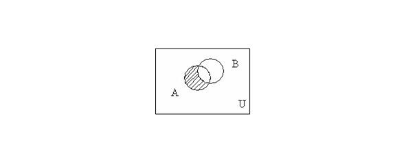
The union of the sets A and B is the set consisting of all those elements that belong to at least one of the sets A, B (Fig. 1.1): A ∪ B = {x | x ∈ A ∨ x ∈ B}.

The intersection of sets A and B is the set consisting of all those and only those elements that belong simultaneously to both the set A and the set B (Fig. & 1.2): A ⋂ B = {x | x ∈ A ∧ x ∈ B}.

The difference between the sets A and B is the set of all those and only those elements A that are not contained in B (Fig. 1.3): A\B = {x | x ∈ A and x ∉ B},

The symmetric difference of sets A and B is the set of elements of these sets that belong either to the set A or to the set B, but do not belong to their intersection (Fig. & 1. 4): A+B= {x | x ∈ A, or x ∈ B, x ∉ A⋂ B},

Absolute complement (negation) of the set A is the set of all those elements that do not belong to the set A (Fig. & 1. 5): ̅A=U\A,

1.4. Set Operations Properties

For arbitrary sets A, B, and C, the following relations are true.

Commutativity of the union: A ∪ B = B ∪ A,

Commutativity of the intersection: A ⋂ B = B ⋂ A,

Associativity of the union: A ∪ (B ∪ С) = (A ∪ B) ∪ С,

Associativity of the intersection: A ⋂ (B ⋂ С) = (A ⋂ B) ⋂ С,

Distribution of the union with respect to the intersection: A ∪ (B ⋂ С) = (A ∪ B) ⋂ (А ∪ С),

Distribution of intersection with respect to the union: A ⋂ (B ∪ С) = (A ⋂ B) ∪ (А ⋂ С),

Laws of action with empty and universal sets: A ∪ ∅ = A, A ∪ A = U, A ∪ U = U, A ⋂ U = A, A ⋂ A = ∅, A ⋂ ∅ = ∅

The law of idempotency of the union: A ∪ A = A,

The law of idempotency of the intersection: A ⋂ A = A,

De Morgan’s laws: A ∪ B = A ⋂ B, A ⋂ B = A ∪ B,

Laws of absorption: A ∪ (A ⋂ B) = A, A ⋂ (A ∪ B) = A,

Gluing laws: (A ⋂ B) ∪ (A ⋂ B) = A, (A ∪ B) ⋂ (A ∪ B) = A,

Poretsky Laws: A ∪ (A ⋂ B) = A ∪ B, A ⋂ (A ∪ B) = A ⋂ B,

Double Supplement Law A=A,

1.5. Euler-Venn Diagrams

The illustrations below are called Euler-Venn diagrams, they can be used to illustrate the equalities sets expressed through given sets, as well as receive new equalities.

1.6. Characteristic functions

1.6.1. Main relations

To prove complex set-theoretic identities, it is more efficient to use characteristic functions.

A characteristic function X_A of the set A ⊆ U is a function defined on the set U with values on the set {0,1}: X_A (x) = {1 if x ∈ A 0 if x ∉ A},

Obviously, the identity L = R will be valid if the characteristic functions of the sets L, Rare equal, i.e.. X_L (x) = X_R (x).

We give the characteristic functions of intersection, union, difference, absolute complement and symmetric difference, as well as an important property of the characteristic functions:

— X_{A ⋂ B} (x) = X_A (x) *X_B (x)

— X_{A ∪ B} (x) = X_A (x) +X_B (x) — X_A (x) *X_B (x)

— X_{A \ B} (x) = X_A (x) — X_A (x) *X_B (x)

— X_A (x) = 1 — X_A (x)

— X_{A + B} (x) = X_A (x) +X_B (x) — 2X_A (x) X_B (x)

— X_A (x) = X²_A (x)

1.6.2. The process of evidence by the characteristic function

To prove the validity of the set-theoretic identities should express the characteristic features of its left and right sides of the characteristic features contained in them sets.

As an example, we prove the validity of one of the laws of action with an empty set: A ⋂ A = ∅.

Using the characteristic functions: X_{A ⋂ B} (x) = X_A (x) *X_B (x), X_A (x) = 1 — X_A (x), we obtain: X_{A ⋂ A} (x) = X_A (x) *X_A (x) = X_A (x) * (1 — X_A (x)) = X_A (x) — X²_A (x) =0

WHAT AND NEEDED TO BE PROVEN.

1.7. Relationships

Relationship is a mathematical structure that formally defines the properties of various objects and their relationships. Relations are usually classified by the number of objects to be linked and their own properties.

An ordered pair (x,y) is intuitively defined as a collection consisting of two elements x and yarranged in a specific order. Two pairs (x,y), (u,v) are considered equal if x=u, y=v and only if. The ordered n-th elements x₁,…,x_n are denoted by (x₁,…,x_n).

The Cartesian product of the sets X and Y is the set X × Y of all ordered pairs (x, y) such that x ∈ X, y ∈ Y.

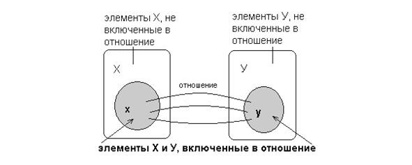
A binary (or two-place) relation R is the set of ordered pairs, a binary relation is a subset of the Cartesian product.

If R is a relation and the pair (x, y) belongs to this relation, then along with the record (x, y) R, the notationis also used xRy. Elements x and y are called the coordinates (or components) of the ratio R.

The domain of a binary relation R is the set D_R= {x ∨ ∃ y, xRy}. The range of binary relations R is the set E_R= {y ∨ ∃ x, xRy}.

Let R XY be defined in accordance with the image in Figure 1.6

The domain of definition of D_R and the range of values of E_{R are} defined respectively: D_R= {x: (x, y) ∈ R}, E_R= {y: (x, y) ∈ R}. The binary relation can be set in any of the ways job sets. In addition, relations defined on finite sets are usually specified: by a

— list (enumeration) of pairs for which this relation is satisfied;

— matrix — the binary relation corresponds to a square matrix of order n, in which the element r_ij, standing at the intersection of the i-th row and the j-th column, is 1 if a_i and a_j is the relation, or 0 if it is absent: R= r_ij, r_ij= [0, (a_i, a_j) ∉ R 1, (a_i, a_j) ∈ R]

1.7.1. Properties of binary relations

— relationship R on the set X is reflexive if for any element xX hRh performed.

— The ratio R for the set X is called anti-reflective (irreflexive) if for any element xX performed ¬ (xRx).

— The ratio R for the set X is symmetric if for all x,x from hRu should be uRh.

— The ratio R for the set X is antisymmetric if for all x, yX of hRu and that x=y.

— A relation R on a set X is called transitive if, for any x, y, z X from xRy, and xRz follows yRz.

A partial order relation R is called linear order if the condition ∀x, y ∈ X: xRy ∨ yRx is satisfied.

A relation R is called a strict order relation on a set Xif it is antireflexive, antisymmetric, and transitive.

Reflective, symmetric, transitive relation on a set X is an equivalence relation on the set X.

Reflexive transitive and antisymmetric ratio is called a partial order relation, or the ratio of the non-strict order on the set X.

If theon the set X relation of partial orderis given ≤, then the set X is called partially ordered. If theon the set X relation of linear orderis given ≤, then the set X is called linearly ordered. If aon a set X relation of full orderis given ≤, then the set X is said to be completely ordered.

Let R — equivalence relation on the set X.

An equivalence class generated by an element x ∈ X is a subset of the set Xconsisting of those elements y X for which xRy. It is designated as: [x] = {y ∈ X | xRy}.

A partition of a set X is a collection of pairwise disjoint subsets of Xsuch that each element of the set X belongs to one and only one of these subsets.

Examples:

1. X= {1,2,3,4,5} Partition: {{1,2}, {3,5}, {4}}.

2. The partition of many students of the institute can be a set of groups.

In other words, a partition of a set X is a family: X = ∪_{i ∈ I}X_i∀i, j X_i ⋂ X_{j j} =0, X_i ⊆ X is an element of the partition.

The set of equivalence classes of elements of any set of X by the equivalence relation R setis the quotient of the set X with respect R denotedand X/R.For example, a plurality of student groups of a given university is a factor in a plurality of a plurality of university students in relation to belonging to one group.

Examples:

— (x, ≤) x ≤ y (x,y) ∈ ≤ — are comparable;

— (x,y) ∉ ≤ — are not comparable.

If (x, ≤), ∀ x ∈ X ∃ a ∈ X ∨ a ≤ x then a is the smallest element. If ∃ a ∈ X ∨ ∀ x ∈ X x ≤ a, then a is the largest element.

Statement: the largest or smallest element is single.

Proof: let a and b be the largest elements in (x, ≤), then ∀ x ∈ X a ≥ x, in particular a ≥ b. Similar to b ≥ a, therefore a=b.

In a similar way, the statement for the smallest elements is proved.

APPROVED PROVEN

1.7.2. Operations on binary relations

Since relations on X are defined by subsets R ⊆ X × Y, the same operations are defined for them as on sets.

— The union R₁ ∪ R₂: R₁ ∪ R₂= {(x,y) | (x,y) ∈ R₁ or (x,y) ∈ R₂}

— Intersection R₁ ⋂ R₂: R₁ ⋂ R₂= {(x,y) | (x,y) ∈ R₁ and (x,y) ∉ R₂}

— Difference R₁/R₂: R₁/R₂= {(x,y) | (x,y) ∈ R₁ and (x,y) ∉ R₂}

— Addition R: R=U/R, where U=M₁×M₂ (or U=M²)

The inverse ratio R^-1:x R^-1y if and only if yRx, R^-1= {(x,y) ∨ (y,x) ∈ R}.

Compound ratio (composition) R1 ∝ R2. Let the sets M₁, M₂ and M₃ and the relationship R₁M₁M₂ and R₂M₂M₃. The composite relation acts from M₁ to M₂ by means of R₁, and then from M₂ to M₃ by R₂, i.e. (a,b) R1 ∝ R2, if there is such an M₂ that (a,c) R₁ and (a,c) R₂.

The transitive closure of R.A transitive closure consists of such and only such pairs of elements a and b from M, that is, (a, b) R, for which in M there exists a chain of (k +2) elements M, k 0 such that a, c₁, c₂, … c_k, b, between whose adjacent elementsis fulfilled R. In other words, ARC₁, with₁RC₂, …, with_kRb.

Two partially ordered sets are called isomorphic if there is a one-to-one correspondence between them that preserves order.

Example: (x, ≤₁), (y, ≤₂) x, y are isomorphic if, where ∃φ:X → Y is a bijective function that preserves order (the definition of a function and a bijective function is given below).

A binary relation is called tolerance if it is reflective and symmetrical. A binary relation is called a quasiorder if it is irreflexive, antisymmetric, and transitive (preorder).

1.8. Functions

A binary relation f is called a function if from (x. y) f and (x. z) f it follows that y=z. Since functions are binary relations, the two functions f and g are equal if they consist of the same elements. The domain of the function is denoted by Df, and the domain is Rf. They are defined in the same way as for binary relations.